🧮 Cracking the Code: Chi-Square Tests in Excel Made Easy! 🎯✨
Hey there, data explorer! 👩💻👨💻
Ever found yourself wondering if your data is following a pattern or just making random decisions? Enter the Chi-Square Test, the ultimate detective for finding out if observed results match expectations. And guess what? You can perform this right in Excel—no fancy tools required! Let’s make it fun, simple, and practical. 🚀
What Is a Chi-Square Test? 🤔
A Chi-Square Test (𝛘²) helps you determine whether the differences between observed and expected data are due to pure chance or something more significant.
Think of it like this:
• Observed Data (O) 🐾: What you actually see (real-world values).
• Expected Data (E) 🎯: What you should see (based on probabilities or assumptions).
If the difference between these two is large, something might be off!
Key Idea:
• Small 𝛘² value? 🟢 The differences are likely due to chance.
• Large 𝛘² value? 🔴 Something unexpected is going on!
When to Use a Chi-Square Test? 🧐
• Your data is categorical (e.g., Yes/No, Red/Blue/Green).
• You want to check if the distribution of categories fits a specific pattern.
• You’re comparing proportions across groups.
Performing a Chi-Square Test in Excel 🖥️
1️⃣ Set Up Your Data
Create two columns:
• One for Observed Frequencies (O) (e.g., the actual number of votes for ice cream flavors like Chocolate, Vanilla, and Strawberry).
• Another for Expected Frequencies (E) (e.g., the votes you expected based on assumptions).
2️⃣ Calculate the Chi-Square Statistic (𝛘²)
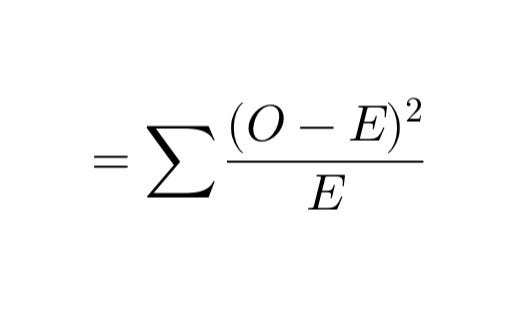
The Chi-Square formula is:
In Excel, break it into simple steps:
1. Calculate the difference: Subtract expected values from observed values (O - E).
2. Square the difference: Use (O - E)^2.
3. Divide by expected value: Divide each squared difference by the corresponding expected value.
4. Add it all up: Sum these results to get the 𝛘² statistic.
Excel formulas to use:
• Difference: =Observed - Expected
• Squared Difference: =(Difference)^2
• Final Step: =SUM(All Results)
3️⃣ Find the Critical Value 📈
Now, compare your Chi-Square value to a critical value from the Chi-Square table. You’ll need:
• Degrees of Freedom (df): This is the number of categories minus 1.
• Significance Level: Usually 0.05 (5%).
In Excel, use the CHISQ.INV.RT function to get the critical value:
=CHISQ.INV.RT(0.05, Degrees_of_Freedom)
If your calculated 𝛘² is greater than this critical value, there’s a significant difference. If it’s smaller, it’s likely due to chance.
4️⃣ Shortcut: CHISQ.TEST Function 🚀
Excel simplifies this process with the CHISQ.TEST function. Here’s how:
• Formula: =CHISQ.TEST(Observed_Range, Expected_Range)
• This directly gives you the p-value.
• If p < 0.05 → Significant difference.
• If p > 0.05 → No significant difference.
Example in Action 🍦
Imagine you’re testing preferences for three ice cream flavors: Chocolate, Vanilla, and Strawberry. You observed the following votes:
• 50 votes for Chocolate
• 30 for Vanilla
• 20 for Strawberry
Your expected votes, assuming equal preferences, are:
• 40 each for Chocolate and Vanilla
• 20 for Strawberry
Using the steps above, you calculate a 𝛘² value of 5.0. With 2 degrees of freedom (3 categories - 1), you compare this to a critical value of 5.99 (at 0.05 significance level). Since 5.0 < 5.99, there’s no significant difference. 🎉
Make It Visual! 📊
Enhance your analysis with a bar chart:
• Plot observed vs. expected frequencies.
• A quick glance will show if something looks off!
Why Chi-Square Is Fun 🥳
Think of it as being a statistical detective:
• You’re spotting differences. 🕵️♀️
• Testing patterns. 🔍
• Solving mysteries in your data. 📖
Wrap-Up
With just a few formulas, Excel makes performing Chi-Square Tests a breeze. Whether you’re analyzing survey results, comparing proportions, or testing distributions, this method empowers you to back your decisions with stats! 💪
Ready to try it yourself? Open Excel and let the detective work begin! 🚀
Have questions? Drop them below—I’d love to hear from you!


