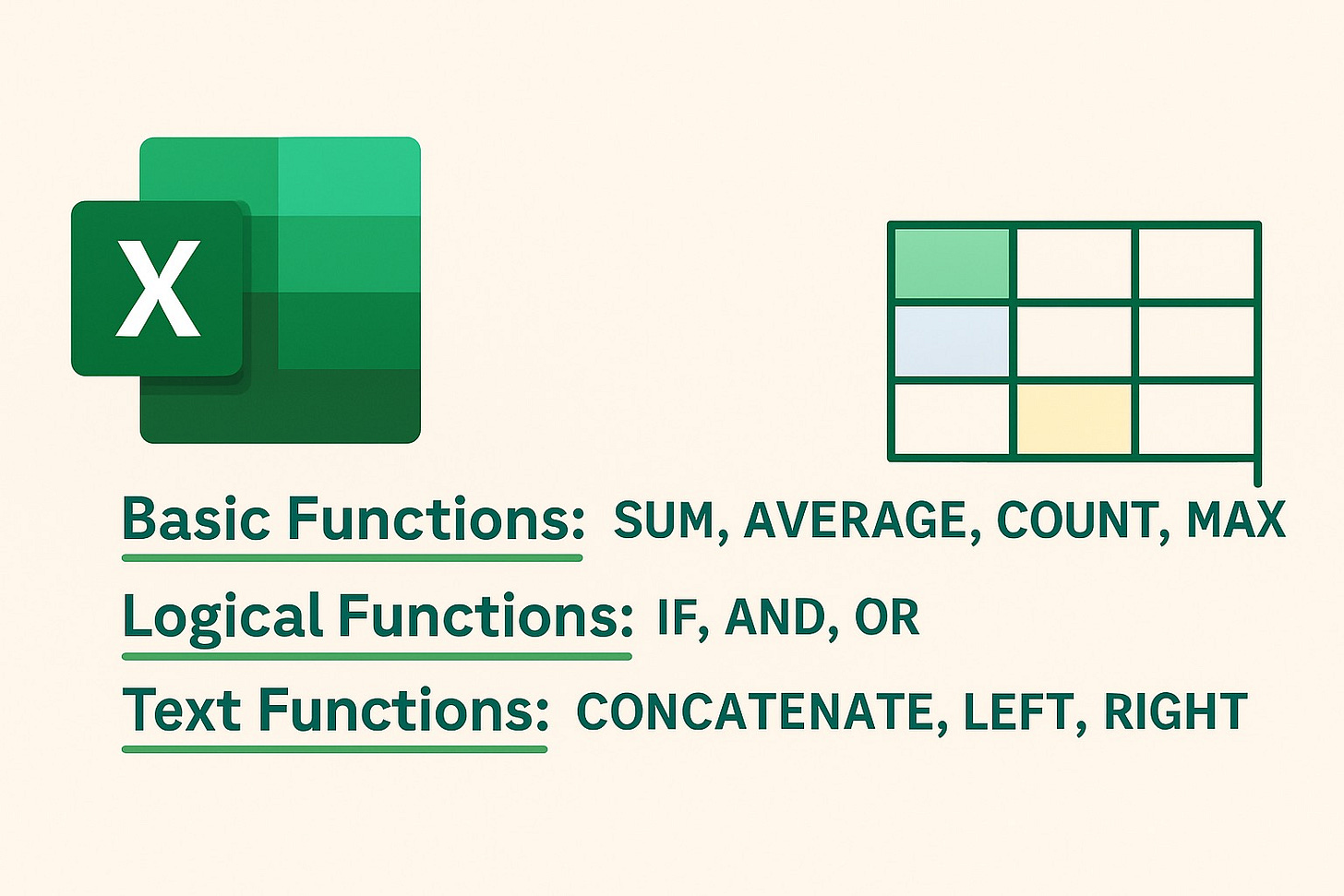
Essential Excel Functions You Should Know
Excel is a powerhouse for data analysis, reporting, and automation. Whether you’re a beginner or an experienced user, knowing the right functions can save you hours of work and boost your efficiency. In this article, we’ll break down some of the most useful Excel functions, explain how they work, and provide plenty of examples.
1. Basic Functions That Make Life Easier
SUM: Adding Up Values Effortlessly
The SUM function adds numbers in a range. It’s one of the most commonly used functions in Excel, helping with everything from financial calculations to inventory management.
Example 1: Adding Sales Data
Let’s say you have daily sales figures in cells B2 to B10 and want to calculate the total sales for the week:
=SUM(B2:B10)
Excel will add all values in the selected range and give you the total instantly.
Example 2: Adding Only Specific Numbers
You can also sum specific numbers instead of a range:
=SUM(100, 200, 300)
This directly adds the numbers provided.
Pro Tip:
If you have blank cells in a column, Excel will ignore them in the SUM function, so you don’t have to worry about errors.
AVERAGE: Finding the Mean Value
The AVERAGE function calculates the mean of a set of numbers. It’s useful for analyzing performance, trends, or any data requiring averages.
Example 3: Finding the Average Score
Imagine you have test scores in C2 to C7 and want to find the average score:
=AVERAGE(C2:C7)
Excel will return the mean of the selected numbers.
Example 4: Ignoring Zero Values
If you have zeros in your dataset and don’t want them included in the average, use AVERAGEIF:
=AVERAGEIF(C2:C7, ">0")
This function calculates the average while ignoring cells with zero values.
COUNT: Counting Numbers in a Range
The COUNT function tells you how many numerical values exist in a given range.
Example 5: Counting Sales Transactions
If you have a column of transaction amounts and want to count how many transactions were recorded, use:
=COUNT(D2:D15)
Excel will count only the numeric entries and ignore blank cells or text.
Bonus:
COUNTA counts all non-empty cells, including text and numbers.
COUNTIF counts based on specific conditions, such as counting how many sales were above $500.
=COUNTIF(D2:D15, ">500")
MAX & MIN: Finding the Highest and Lowest Values
MAX returns the largest number in a dataset.
MIN returns the smallest number.
Example 6: Identifying the Best and Worst Performers
If column E contains employee sales numbers, you can find the top performer’s sales using:
=MAX(E2:E20)
And the lowest sales using:
=MIN(E2:E20)
These functions help in performance analysis, stock tracking, and business intelligence.
2. Logical Functions for Smarter Decisions
IF: Automating Decision-Making
The IF function is one of the most powerful functions in Excel. It allows you to return different values based on a condition.
Example 7: Checking Pass or Fail
If students’ scores are in F2 to F10 and the passing mark is 50, you can use:
=IF(F2>=50, "Pass", "Fail")
This formula will return Pass if the score is 50 or above; otherwise, it will return Fail.
Example 8: Assigning Discounts Based on Purchase Amount
If a customer spends $500 or more, they get a 10% discount; otherwise, no discount:
=IF(G2>=500, G2*0.9, G2)
This formula calculates the discounted price for qualifying purchases while keeping others unchanged.
AND & OR: Combining Multiple Conditions
AND checks if all conditions are true.
OR checks if at least one condition is true.
Example 9: Determining Bonus Eligibility
Let’s say employees get a bonus if they meet two conditions:
Sales must be above $5000
Customer ratings must be above 4
Use:
=IF(AND(H2>5000, I2>4), "Eligible", "Not Eligible")
Example 10: Checking Eligibility for a Loan
If a customer is eligible for a loan if they either have a high credit score (750+) OR a stable income ($50,000+), use:
=IF(OR(J2>=750, K2>=50000), "Eligible", "Not Eligible")
3. Text Functions for Managing and Cleaning Data
CONCATENATE (or TEXTJOIN in Newer Excel Versions)
This function combines text from multiple cells into one.
Example 11: Combining First and Last Names
If first names are in A2 and last names in B2, use:
=CONCATENATE(A2, " ", B2)
This will return “John Doe” if A2 contains John and B2 contains Doe.
Example 12: Combining City and Postal Code
If cities are in C2 and postal codes in D2, use:
=TEXTJOIN(", ", TRUE, C2, D2)
This will return “Auckland, 1010” instead of manually entering them.
LEFT & RIGHT: Extracting Specific Text
LEFT pulls characters from the start of a text.
RIGHT pulls characters from the end.
Example 13: Extracting Country Codes from Phone Numbers
If column E contains phone numbers formatted as +64 987654321, you can extract the country code:
=LEFT(E2, 3)
Example 14: Getting the Last 4 Digits of an ID
If IDs are in column F, and you need the last 4 digits:
=RIGHT(F2, 4)
Some Newer Excel Updates You Might Have Missed
TEXTSPLIT & TEXTJOIN: Newer alternatives for handling text more efficiently.
XLOOKUP: A more powerful replacement for VLOOKUP with improved flexibility.
LET Function: Allows defining variables inside a formula to optimize calculations.
Excel functions simplify tasks, enhance productivity, and reduce errors. Whether you’re dealing with numbers, making decisions, or managing text, these functions can significantly improve your workflow.
Which Excel function do you use the most? Let me know in the comments!


