
Excel Basics: Formatting, Shortcuts, and Navigating Like a Pro

Excel is an essential tool for business analysis, financial modeling, and data organization. Whether you’re crunching numbers, creating reports, or handling large datasets, understanding Excel’s formatting, shortcuts, and interface can make your work more efficient. Let’s break down these topics with clear explanations, practical examples, and some lesser-known tips.
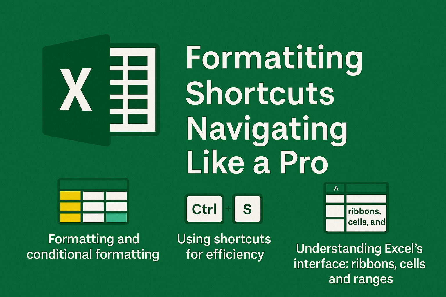
Formatting and Conditional Formatting: Making Data Visually Impactful
Why Formatting Matters
Formatting helps structure your data so that it is clear, easy to read, and visually appealing. Imagine receiving a messy spreadsheet with no alignment, inconsistent fonts, and unformatted numbers. It would be difficult to interpret the data quickly. Proper formatting ensures clarity, professionalism, and better data analysis.
Common Formatting Options
Number Formatting – Excel allows you to change the appearance of numbers without altering the actual value. Some common options include:
Currency
Percentage
Date and Time
Custom Formats
Example: If you enter “2500” in a cell and apply the currency format, it will be displayed as “$2,500.00” while keeping the actual value 2500.
Font and Alignment – Adjust font styles, bold important headings, and center-align data for a structured look.
Borders and Cell Colors – Use borders to separate sections and fill colors to highlight key figures.
Merging and Wrapping Text – Merging combines multiple cells, while wrapping ensures long text is fully visible within a cell.
Conditional Formatting: Highlight What Matters
Conditional Formatting is a powerful feature that applies formatting automatically based on certain conditions.
Common Uses:
Highlighting values above or below a threshold
Identifying duplicates
Color-coding data based on specific criteria
Example 1: Highlighting High Sales Figures
If you want to highlight sales figures greater than $10,000:
Select the range of sales data.
Go to Home > Conditional Formatting > Highlight Cells Rules > Greater Than
Enter 10000 and choose a formatting style (e.g., green fill).
Now, any sales figure above $10,000 will be automatically highlighted in green.
Example 2: Color-Coding Dates
If you want overdue tasks (past today’s date) to appear in red:
Select the column with dates.
Choose Conditional Formatting > New Rule > Use a Formula
Enter the formula: =A1<TODAY()
Choose red fill for overdue dates.
This makes it easy to spot overdue tasks at a glance.
Using Shortcuts for Efficiency: Work Faster, Not Harder
Excel is packed with keyboard shortcuts that can significantly speed up your workflow. Instead of navigating through menus, mastering a few key combinations can save you time.
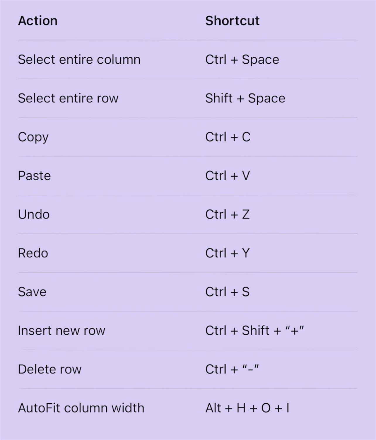
Essential Shortcuts to Know
Example: Fast Data Entry with Autofill
If you need to enter a sequence of numbers, dates, or formulas, use the Autofill Handle:
Enter the first value (e.g., 1 in cell A1).
Click the bottom-right corner of the cell and drag down.
Excel will automatically fill the series (1, 2, 3…).
For advanced users, Ctrl + D fills data down, while Ctrl + R fills data to the right.
Understanding Excel’s Interface: Ribbons, Cells, and Ranges
Before diving deeper into Excel, let’s get comfortable with its interface.
The Ribbon: Your Control Panel
The Ribbon is the menu bar at the top, organized into tabs such as:
Home: Basic formatting, alignment, number formatting
Insert: Charts, tables, pivot tables
Formulas: Functions and calculations
Data: Sorting, filtering, data tools
Review: Spelling, comments, protection
View: Page layout, zoom, freeze panes
Cells, Rows, and Columns
Cell: The basic unit in Excel (e.g., A1, B5).
Row: A horizontal group of cells, identified by numbers.
Column: A vertical group of cells, identified by letters.
Example: If you type “Sales” in A1 and “Revenue” in B1, these two are adjacent cells.
Understanding Ranges
A range is a selection of multiple cells, such as A1:A10 or A1:D10. Ranges can be used in formulas, formatting, and charts.
Example: Selecting a Range for Formatting
If you want to bold all column headers in row 1, select A1:D1 and press Ctrl + B.
Latest Updates in Excel: What’s New?
Microsoft frequently updates Excel with new features to enhance productivity. Here are a few recent additions:
1. Dynamic Arrays (Newer Versions of Excel)
Excel now allows formulas that spill over multiple cells. For instance, the SORT function can arrange data dynamically:
=SORT(A1:A10,1,TRUE) will automatically sort values in ascending order.
2. XLOOKUP (Replacement for VLOOKUP and HLOOKUP)
XLOOKUP is more flexible and efficient than VLOOKUP:
It searches both horizontally and vertically.
It eliminates the column index number problem.
It works even if columns are moved.
3. Data Types Integration
Excel now connects to live data sources, providing real-time updates for stocks, geography, and even LinkedIn data.
Pro Tips for Working Smarter in Excel
Use Named Ranges – Instead of referring to A1:A100, assign a name (e.g., “SalesData”) for clarity in formulas.
Freeze Panes for Better Navigation – If you’re working with large datasets, go to View > Freeze Panes to keep headers visible while scrolling.
Use Format Painter – Quickly copy formatting from one cell to another by clicking Format Painter in the Home tab.
Convert Data into a Table – Press Ctrl + T to convert a dataset into a structured table, making sorting and filtering easier.
Use Data Validation – Restrict input to specific values (e.g., dropdown lists) to maintain data accuracy.
Mastering Excel’s basics—formatting, shortcuts, and interface navigation—lays the foundation for more advanced functions like pivot tables, macros, and automation. The more you practice, the faster you’ll get. Excel is not just about number crunching; it’s about presenting data in a meaningful way.